
Pressure-sensitive adhesives (PSAs) are commonplace in our everyday lives.1-2Surgical tape, box-sealing tape and self-stick products such as adhesive stamps and removable adhesive notes are just some of the consumer products that use pressure-sensitive adhesives. PSAs are used in space and automotive applications as well.
Pressure-sensitive adhesives are generally coated onto a backing material such as paper, cloth or polymers to support the thin adhesive layer. They adhere to surfaces with minimal applied pressure, remain tacky at room temperature, do not chemically react, and can be cleanly removed from a surface.
Because of their variety of end uses, PSAs are applied in a range of operating temperatures and conditions. No theory has been able to predict a priori the behavior of a PSA based on the properties of the adhesive and substrate.3 Therefore, multiple testing must be performed. One of the most common tests is the peel test. The peel force measured is not an inherent property of the adhesive, but depends on many variables, such as the test method, temperature, peel rate, degree of contact, adhesive chemistry and thickness, aging, adhesive backing, and the substrate. Common peel tests include the T-peel test, the 180° peel test, and the 90° peel test.4-5
Figure 1 illustrates a 90° peel-force measurement, where the measured peel force, normalized by width of the tape, is shown as a function of peel length. The normalized peel force increases from zero to a steady peel force within 2 mm. Data from the first 2.5 cm of the peel are generally rejected, and the next 5 cm of the results are evaluated to give an average peel force.2 We will define this average peel force measurement as the macroscopic average peel force.
Peel tests are often performed at various testing speeds and temperatures while keeping many other experimental parameters constant, such as the adhesive chemistry and thickness. The Williams, Landel and Ferry (WLF) time-temperature superposition equation enables a set of peel force curves measured at various frequencies or temperatures to be reduced to a single master curve (see Figure 2).6-7 The peel rate increases from left to right on the graph, whereas the temperature increases from right to left. At very low temperatures (high peel rates), unsteady (shocky) peel is observed. As the temperature is increased, a region of steady (smooth) peel with clean interfacial adhesive failure occurs. For crosslinked adhesives, the peel force continues to decrease with increasing temperature. For uncrosslinked adhesives, another transition occurs at higher temperatures (low peel rates) characterized by a change from interfacial failure to cohesive splitting of the adhesive, leaving residue on the tape and the peel surface. The peel force often increases at this transition, followed by another region of decreasing peel force with increasing temperature. The peel force master curve identifies the best operating conditions for an adhesive. Because many peel tests are performed at various peel rates or temperatures, obtaining a peel force master curve can take a day or more. Measurement of the peel force as a function of temperature alone can provide much of the general characterization information of the master curve and allow a comparison of adhesives. The information about the relationship between temperature and peel rate contained in the shift factor is not obtained by this means, however. Often, peel forces are measured at one standard peel rate, and the adhesive performance is inferred from these results.

Faster is Key: High-Throughput Methodology
To alleviate the extensive testing required to produce a peel force master curve, we have applied high-throughput methodology to the peel test. High-throughput methodology challenges standard practices by developing procedures and measurement methods that can be performed faster yet give similar information. In this case, instead of measuring multiple peel tests at each desired temperature, we measured the peel force from a surface that varied linearly in temperature across the surface. As the tape is peeled, the adhesive is peeled from the surface at a different temperature. Since we can correlate temperature with peel distance, we are able to determine the temperature dependence of the peel force with one peel test.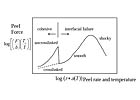
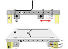

The plate was bolted onto the movable stage of a texture analyzer (Texture Technologies Corp., Scarsdale, NY). The texture analyzer was configured to measure the tensile force at a 90° angle to the stage. The movable stage allows the 90° angle to be maintained as the tape is pulled from the surface.
The stainless-steel gradient plate was cleaned according to ASTM recommended cleaning procedures: wash three times with diacetone ether and dry with a tissue after each wash.5 This was followed by washing three times with acetone, again drying with a tissue after each wash.
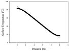
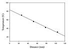
The plate was then allowed to reach equilibrium temperature by heating one end of the plate and cooling the other end for two hours prior to testing.
After the plate had equilibrated for two hours, a 1.9 cm strip of PSA tape was applied to the gradient plate using a 2 kg rubber roller. The adhesive tape (Scotch® Box Sealing Tape 353, 3M, St. Paul, MN) is a commercially available rubber resin adhesive tape. The nominal adhesive thickness is 25 µm. The adhesive is supported on a biaxially oriented polyester backing which has a thickness of 23 µm. The "hot" end of the tape is clamped by a metal grip on the texture analyzer. The adhesive was peeled from the plate at a rate of 0.14 mm/s. The tape was peeled less than 5 minutes after the PSA tape was applied to the surface.

The results presented in Figure 6 demonstrate that the temperature dependence of the peel force can be determined in one peel test. Multiple peel tests at different temperature ranges can be combined to give a peel force master curve over a larger temperature range. In addition, the WLF equation can be directly tested on peel measurements by comparing the peel forces measured in the high-throughput technique and those predicted by the WLF equation. Future experiments will investigate this question.
Benefits and Opportunities of High-Throughput Peel Testing
The results presented demonstrate that accurate peel testing can be achieved using a gradient temperature plate. The gradient temperature plate can be tailored to any temperature range or peel rate desired. Not only can peel force measurements be obtained more quickly, but peel transition temperatures can easily be determined.High-throughput testing allows faster screening of adhesives, which will influence the direction and pace of product development. A number of other peel force variables can also be investigated using high-throughput methodology, including measuring the peel force as a function of a continuously varying peel rate or as a function of adhesive thickness.12-13
Acknowledgements
P.M.M. would like to thank John Johnston, Don Hunston, M. Chiang and A. Kinloch for helpful discussions.For more information on other high-throughput measurements in materials science, visit the N.I.S.T. Combinatorial Methods Center at http://www.nist.gov/combi.
Note: Certain commercial equipment, instruments, or materials are identified in this paper in order to adequately specify the experimental procedure. Such identification does not imply recommendation or endorsement by the National Institute of Standards and Technology, nor does it imply that the materials or equipment identified are necessarily the best available for the purpose.

