

Editor’s note: This paper was awarded the Pressure Sensitive Tape Council’s 2012 Carl A. Dahlquist Award for Best Technical Paper.
One of the factors defining the adhesive properties of polyacrylate-based pressure-sensitive adhesives (PSAs) is the composition of comonomers constituting the polymeric backbone. Nuclear magnetic resonance (NMR) spectroscopy, particularly 13C NMR, is widely accepted as an appropriate method for determining comonomer composition of acrylic copolymers. However, for a number of reasons, 13C NMR is not the method of choice for routine analysis requiring prompt results.
Prior to NMR investigation, dry polymeric samples need to be dissolved. Depending on the sample’s molecular weight, this process could require anywhere from a few hours to a couple of days. Chemically crosslinked samples do not dissolve, but form swollen gels, often entrapping air bubbles. Thus, in order to avoid adverse effects on the spectra quality, these air bubbles must be removed by centrifugation prior to measuring. Additives like tackifier resins sometimes complicate the spectra and should be removed in preceding purification steps.
For quantitative evaluation, a good signal-to-noise ratio, sufficient relaxation time and avoidance of unwanted nuclear Overhauser effects (NOEs) are necessary. Running times for 13C NMR spectra are therefore approximately 12 hours. This is true even when relaxation agents like chromium acetylacetonate are used. Nonetheless, a high degree of crosslinking restricts the achievable spectral resolution, which may in turn cause a loss of accuracy in quantification.
The evaluation of a 13C NMR spectrum requires a person skilled in the art who also has extended practical experience. As such, a comonomer analysis of an acrylic PSA via 13C NMR is typically takes more than one day.
IR Spectroscopy
Infrared (IR) spectroscopy is a suitable and widely used analytical tool for routine analysis in quality control or failure analysis, where results are usually required quickly. The conformity of an unknown sample with a reference sample is easily assessed by visual spectra comparison, resulting in two categories: IR-identical or not IR-identical. Possible reasons for IR non-identity could be wrong monomers or monomer ratio, or undesired sample contamination. Since the IR spectra of polyacrylates look quite similar at first glance, the interpretation of the root cause for the deviation is not trivial.
When certain peaks or bands are characteristic for specific components, IR spectroscopy can be used for quantitative analysis of two- or multi-component systems. With a chemometric model once created, the evaluation of the IR spectrum of an unknown sample is quick and easy. A chemometric model is usually built with statistical modules, which are part of state-of-the-art IR spectrometer software packages.
The objectives of the present work are to investigate IR spectroscopy as an alternative analytical path to quantitative comonomer determination of polyacrylate-based PSAs. This will be achieved through the comparison of chemometric modeling to 13C NMR spectroscopy, with respect to accuracy, precision and limitations.
IR Spectra of Acrylic PSAs
Acrylic PSAs are typically copolymers that are composed of a mixture of different acrylic acid or methacrylic acid alkyl esters, sometimes containing non-acrylic comonomers like vinylacetate or styrene. The number of C atoms of the alkyl group has a strong influence on the glass-transition temperature (Tg) of the respective homopolymer. One of the prerequisites for pressure-sensitive adhesion is a Tg far below the desired temperature of bond formation, which is typically in the range of 30-70°C. With commercially available monomers, this is achieved mainly with n-butyl acrylate (n-BA) and/or 2-ethylhexylacrylate (2-EHA), exhibiting homopolymer Tgs of 43 and 58°C, respectively.
In order to balance good bonding and debonding properties, comonomers like methyl acrylate, methyl methacrylate, ethyl acrylate, stearyl acrylate, or voluminous species like isobornyl acrylate and t-butyl acrylate are frequently included, usually in a minor portion. Acrylic acid is also widely used to increase cohesion and Tg and serve as a functional monomer for chemical crosslinking. The latter function can also be fulfilled by monomers carrying hydroxyl groups, like 2 hydroxyethyl acrylate.1,2
The IR-ATR spectra of the homopolymers of the most common monomers (n-BA and 2-EHA), as well as a binary copolymer of the two monomers in equal ratio, were studied. As expected, the spectra look essentially similar at first glance. However, a more detailed inspection reveals differences in the band interval between 3,000 and 2,800 cm-1 (CH stretching vibrations), and, to a minor extent, in the fingerprint region between 1,500 and 700 cm-1.
Differences in peak occurrence and peak intensity are clearly identifiable upon investigation. The peak area in the CH stretching region of n-BA is significantly smaller than that of 2-EHA, reflecting the different size of the alkyl group contributing to the band intensity. Furthermore, the branched 2-EHA side chain has an additional peak at 2,860 cm-1, which is not present with that of the linear n-BA.
It is clear that additional components significantly increase the spectrum complexity. Thus, it is fair to state that evaluation by visual inspection is not a viable approach. Instead, distinctive characteristics better allow for a quantitative calibration model approach.
Multivariate Calibration
As outlined above, different acrylate monomers and monomer compositions cause significant and reproducible differences in the corresponding IR spectra. Inversely, from a given spectrum, the corresponding monomers can be derived. The spectral variance between different acrylates is not located in just one single peak, but in broad and partly overlapping peak intervals. In this case, a potent predictive model can only be designed by means of multivariate statistics.
In multivariate calibration, a mathematical model is developed that translates spectral information (factors) into chemical information (responses). Numerous methods are employed in multivariate statistics. For linking spectral data with chemical composition, the partial least square (PLS) regression method turned out to be particularly suitable. From the mathematical perspective, the spectral data and the concentration data are converted into the form of matrices. Each row in the spectral data matrix refers to a sample spectrum. The matrices are then broken down into their Eigenvectors, which are called factors or principal components.
The most beneficial aspect of this approach is that the relevant spectral features can be accurately described with relatively few factors. Some of these vectors simply represent the spectral noise of the measurement, and thus can be neglected. The original spectral data is so reduced to just the relevant principal components, therefore leading to a considerable reduction in data extent. By employing a PLS regression algorithm, the best correlation function between spectral and concentration data matrix can be found.
The Quant module of the Bruker Opus software uses PLS regression. The focus of this work was the development and validation of a predictive model using a given statistical process according to the Opus software. Detailed information on the mathematical background of PLS regression can be found elsewhere.3,4
Experimental
Three grams of acrylate monomer were mixed with 7 g ethyl acetate, including 0.1% radical initiator Vazo 67 (Pergan, Germany) in a 20 ml GC vial. The oxygen was then removed from the reaction mixture by aerating with nitrogen gas for 5 minutes. The vials were kept in a water bath for 5 hours at 60°C.
When synthesizing copolymers with considerably different polymerization parameters (acrylates vs. methacrylates vs. vinyl acetate), the reaction time was extended to 48 hours in order to achieve a conversion close to 100%. For copolymers containing vinyl acetate, a residual monomer analysis by gas chromatography was performed, and the real vinyl acetate concentration was calculated. The solvent and residual free monomers were first evaporated at room temperature for 3 hours, followed by 2 hours drying at 120°C in an oven.
Purification of Polyacrylate Polymers
For the removal of tackifier resins, 100 mg of the crosslinked sample polymer was placed in a centrifuge tube and 5 ml of acetone was added. This mixture was agitated at room temperature for 12 hours, the extracted gel centrifuged and the acetone decanted. The gel was then washed two times with 5 ml of fresh acetone, centrifuged and finally dried in an oven for 2 hours at 80°C.
For mineralic filler removal, the acrylic polymer solution was diluted to approximately 10% solid contents. The low viscous solution was then centrifuged until the filler was completely precipitated and the supernatant clear liquid decanted. The solvent was then evaporated in an oven.
IR Spectroscopy
The IR spectra were recorded on a Bruker Vertex 70 FTIR spectrometer, equipped with a diamond ATR device (Golden Gate, Bruker). The absorption was measured in a wave number range from 4000-400 cm-1. For a spectrum, 64 scans were taken, with a baseline correction also carried out. The sample polymers all had PSA properties and were brought into intimate contact with the diamond crystal of the ATR unit by gentle finger pressing action. Every calibration sample was recorded twice in order to consider reproducibility.
NMR Spectroscopy
About 300 mg of the copolymer were dissolved in 2.5 ml deuterated chloroform (CDCl3), containing 10 mg/ml chromium actylacetonate. 13C NMR spectra were acquired under TOPSPIN 2.1 (Bruker Biospin GmbH, Rheinstetten) on a 300 MHz Bruker Avance III spectrometer, equipped with a 10 mm broadband probe. The temperature was set to 300 K.
An inverse gated decoupling sequence was chosen, and 32,000 data points were recorded. The overall relaxation time was set to 5 s. Usually, 8,000 scans were recorded to ensure a sufficient signal-to-noise ratio for quantification. Prior to Fourier transformation, the FID was zero filled to 64,000 data points and multiplied by an exponential function with a line broadening factor of 1 Hz. The integration of the NMR signals was accomplished after thorough baseline correction.
Results and Discussion
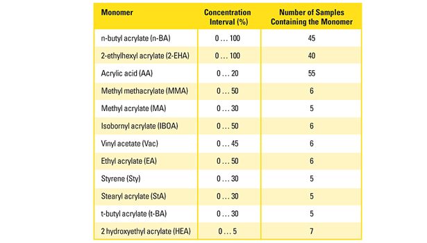
A sufficient amount of information in terms of IR spectra of the calibration polyacrylates must be provided to properly build the predictive model. For this purpose, more than 60 polyacrylates with defined comonomer composition were synthesized according to concentration intervals of the individual monomers, as they are typically found in PSA. Table 1 summarizes the monomer selection, the chosen concentration intervals and the number of calibration polymers containing the respective monomer species.
The most important monomers (n-BA and 2-EHA) were present from 0-100%; all others up to a maximum of 50%. The monomer compositions were uniformly distributed over the whole concentration range. For practical reasons, the number of calibration samples containing monomers of minor importance was rather low (5-7). This lack in accuracy was partly compensated by a multiple of zero concentration samples.
Setup of the Calibration Model
The key tool for the chemometric modeling procedure in the present work is the Quant 2 calibration software, which is part of the IR spectrometer software package Opus, Bruker Optik GmbH (here version 6.5).5 As soon as the ATR IR spectra of the different calibration polymers with defined composition are recorded, calibration of the model can start.
The first step is defining the components (the monomers). Both the spectra and the corresponding comonomer compositions are included in the calibration method. For calculating the first model, the whole spectra with no spectral data preprocessing are applied. The first unrefined model has to be evaluated to test its reliability of prediction (validation). Generally, two methods of validation are used: test set and cross validation. The first requires two sets of samples: the calibration set (first) and a validation set (second).
In this experiment, since the number of available calibration samples for practical reasons is limited, the cross validation approach was preferred. Here, one sample is taken out of the entity of calibration samples and used for validation. With the remaining samples, the composition of the validation sample is calculated and compared with the true values. This procedure is repeated until all samples have been used for validation.
As a result, a coefficient of determination (R2) and the root mean square error of cross validation (RMSECV) can be calculated. These figures give information about the predictive quality of the model (true vs. calculated values). The better the model, the more R2 approaches its limiting value of 100%. The RMSECV reflects the size of the prediction error. The better the model, the more RMSECV approaches a limiting value of 0. It is considered to be the most meaningful criterion for the predictive power of a model. The RMSECV is dependent on the rank of the model. The rank is the number of factors which are used by the model. As mentioned above, the factors differ in their contribution to spectral information. Only the most significant factors are needed to explain the spectral features of the components. There is typically an optimum number of factors, where enough spectral information is considered for a good prediction while spectral noise is excluded. The optimum rank is connected with a minimum RMSECV value. In the chosen rank, possible outliers should be removed. This can change the optimal rank. The validation thus needs to be repeated after outlier removal.
The model quality can usually be further improved after the first validation step by selecting the most important frequency ranges and by spectral data preprocessing. Visual inspection of the spectra sometimes gives indications as to which frequency range reflects the structural variance most. Sometimes, more than one region shows a strong spectral response (e.g., in the CH stretching and the fingerprint region). Selecting those frequency intervals is another measure to concentrate on the most useful spectral information and to exclude spectral noise. With advanced settings, the validation step is repeated and the success monitored via the RMSECV value at the optimum rank. After the minimum RMSECV has been found by narrowing down the frequency intervals, a further refinement of the model may be possible by applying spectral data preprocessing.
Repeated measurements of the same sample do not often result in fully congruent spectra. In order to include the spectral variance, all calibration samples are recorded at least twice. A further reduction of the adverse effect of spectral fluctuations can be achieved by mathematical operations, leading to a normalization of the spectra. Numerous operations, such as first or second order derivation, vector normalization or minimum/maximum normalization, are possible. No general guideline can be given regarding which method is best suited. Again, the impact on the RMSECV value reflects the success of the model refinement. Thus, the model refinement is a trial-and-error approach.
In the Quant 2 program, an optimization tool may be used to support the model refinement. As a result, the RMSECV value and the rank are obtained for numerous frequency intervals and data preprocessing modes. This tool is particularly helpful for defining the optimal frequency ranges. The definition of the preferred parameters is done by the experimenter. With the optimized parameters, the chemometric model is finished and is ready to be applied on spectra of unknown composition.
Comprehensive Calibration Model
The number of components in the response can be defined in the validation step. If all the components are selected, the model gives a total comonomer analysis of the unknown sample. At first glance, such a kind of comprehensive calibration model is a favorable approach. However, the limitations become obvious during refinement of such a model. As outlined above in the refinement step, outliers are eliminated and frequency intervals as well as spectral data preprocessing selected.
For the 12 acrylate monomers considered in the model, all three refinement variables are partially—if not entirely—different. As a consequence, the degrees of freedom in optimization are limited: the improvement for one component often impairs the predictability of others. It was impossible to find parameters where all R2 and RMSECV values were acceptable. This is due to the fact that the distinctive features of the different monomers are located in different spectral regions, and no shared narrow spectral interval is relevant for all monomers in equal measure. Thus, the means of model refinement cannot be fully exploited with this approach.
Individual Calibration Models
The opposite extreme is to select only one component in the validation step and to refine the model for one individual monomer at a time. According to this approach, 12 individual calibration models are obtained that can be applied to an unknown sample in parallel. Finally, 12 single results give the desired information with a maximum level of accuracy since, for every monomer, the optimal outlier elimination, frequency intervals and data preprocessing can be worked out without any interference with other components. Table 2 shows the optimization results in terms of frequency intervals, rank, R2 and RMSECV values.
The selected frequency intervals for the 12 monomers in total cover nearly the whole mid-IR frequency range. Monomers with long alkyl chains like n-BA, 2-EHA and StA are mostly present in the CH stretching region, alkyl acrylates with smaller alkyl chains occur more in the fingerprint region. For monomers with special structural elements like AA (carboxyl function) and Sty (aromatic ring), unique and characteristic frequency intervals are recognized as specific: around the carbonyl peak of AA at 1,692 cm-1 and the aromatic ring out-of-plane vibrations at 695 cm-1.
The R2 in most cases is higher than 98% and the RMSECV is below 1.
Verification of the Model
Verification GuidelinesLimits of Quantification
|
The significance thresholds and the accuracy of prediction were determined by comparing the results of the chemometric model with the nominal monomer concentrations. The importance of this verification becomes especially clear for zero concentrations; here, the model response usually is not exactly zero but plus/minus some percentage. Hence, a guideline is needed to distinguish between significant values and noise. The limits of quantification, the accuracy of prediction for the different monomers and the significance interval of the total of determined monomers are summarized in the sidebars.
The significance threshold for all monomers is 5%. The exceptions are AA (3%) and n-BA (10%). This means that a model response above the limit of quantification is a clear indication for a monomer’s presence. Thus, values far below more than likely indicate noise.
The extraordinarily high uncertainty for n-BA is a consequence of the relatively low coefficient of determination R2 (97%) or high RMSECV, respectively (3.9). It is assumed that the stronger 2-EHA response in the CH stretching region, overlapping with n-BA peaks, causes this uncertainty.
Usually the single monomer contents do not sum up to exactly 100%. A tolerance of ± 8% proved to be the valid range. Responses beyond this corridor indicate an invalid result. The most likely reason is a sample outlying the scope of the model.
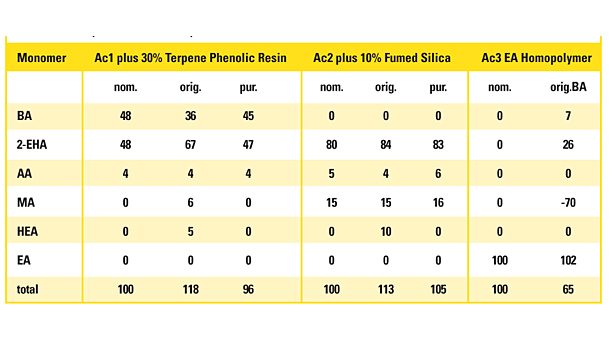
These limiting factors are essential for interpreting model results and to deduce the “real” monomer composition from the calculated crude model responses. Table 3 displays the analysis result of an acrylic PSA and the adjusted result after applying the rules listed in the sidebar compared to the nominal monomer concentration as an example.
The three major monomers, all of them far above the significance threshold, are well predicted. Though perfectly recognized by the model, the minor monomer HEA is below the limit of quantification of 5% and is thus not included in the adjusted result. It may be regarded as a hint of this monomer’s presence, but it is statistically not assured. Thus, the limit of detection is below the limit of quantification. Neither the model result nor the adjusted result adds up to exactly 100%. As 96% lies well within the corridor of 92 and 108%, the result is plausible.
Model Limitations
|
Accuracy of Prediction for Proven Monomers
± 3 percentage points for monomer contents < 20% (except AA) ± 6 percentage points for monomer contents > 20% (except AA) ± 2 percentage points for AA contents < 20%
Significance Interval of the Total of the Determined Monomers 100 ± 80% |
The three samples as received for analysis are outlying the tolerance interval of the total of the determined monomers (100% ± 8%), indicating that their composition is not covered by the model. Ac1 contains 30% by weight of a terpene phenolic tackifier resin. It is plausible that the spectrum is influenced by this substantial amount of additive. The resin contributes to the intensity in the CH stretching band. Consequently, the model, focusing on this band for the acrylates with longer alkyl chain, recognizes a higher portion of n-BA and 2-EHA compared to the pure polymer.
The polymer Ac2 was mixed with 10% by weight with fumed silica as a mineralic filler. It has a strong absorption below 1,250 cm-1. The calibration model for HEA concentrates exclusively on the frequency interval 1,140-780 cm-1. Therefore, the silicate material simulates the presence of HEA. Other monomers are not affected.
The model prediction of the EA homopolymer Ac3 is far out of the tolerance interval, as the model was built with a maximum EA comonomer content of 50%. These examples show that the model is sensitive to samples outside of the calibration scope and indicates this by results outside of the tolerance interval. If the result is close to the tolerance limits, doubts about its validity can be ruled out by visually comparing the IR spectrum with the calibration spectrum of the nearest composition.
Comparison of Comonomer Analysis with IR and NMR
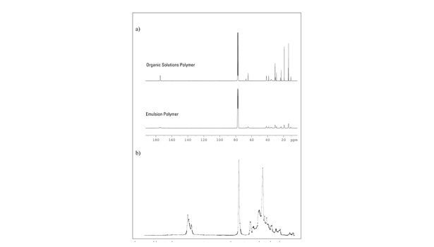
Figure 1 shows two 13C NMR spectra of polyacrylates (nominal comonomer composition: n-BA:2-EHA: AA = 67:30:3) that differ in the polymerization method: free radical organic solution polymerization vs. emulsion polymerization. In contrast to the solvent-borne polymer, the emulsion polymer exhibits a high degree of intraparticle crosslinking. The spin-spin relaxation time (T2) is shortened due to restrictions in the polymer chains’ mobility. This causes significant peak broadening and, in some cases, signal overlapping.
As a consequence, crosslinking may affect precise integration. This is especially true for the quantification of AA, which becomes more uncertain as it is determined indirectly by subtraction of the entity of the carbonyl C-atoms from the entity of the esterified C atoms. This also applies to acrylic polymers crosslinked by polyvalent metal salts, the use of chemical crosslinkers or irradiation-induced crosslinking.
In contrast, the corresponding IR spectra are identical. The IR active vibrations take place on the scale of a few atoms and are not affected by crosslinking. For quantifying the AA, the IR calibration model uses (among others) the AA specific carbonyl peak at 1,692 cm-1. Thus, this direct determination is especially precise. Additives in negligible amounts (such as crosslinkers and antioxidants that are usually used in amounts between 0.1-2%) do not interfere with the IR chemometric model, since they do not or only marginally appear in the IR spectra.
For comonomer analysis via 13C NMR spectroscopy, a typical tolerance is 15% relative error for minor monomer concentrations down to 5% relative error for major ones. These figures are certainly influenced by signal-to-noise ratio, spectral resolution, presence of foreign matter and other adverse factors. The limit of detection is typically 1-2%. This means that, on average, the uncertainty of the IR model presented here is twice as much as that of 13C NMR spectroscopy. For single-digit monomer concentrations, the 13C NMR has a clear advantage in accuracy except for AA as outlined above. This is not a general rule but refers to the performance of the model presented in this work. It is a question of balancing the desired model performance with the labor of creating calibration samples.
Conclusion
Chemometric comonomer analysis of polyacrylates with the aid of an IR calibration model proved to be feasible for a defined scope of monomers and comonomer compositions. The model’s quality in terms of prediction accuracy is influenced by the number of calibration samples used for building the model. While creating the chemometric IR model requires expert knowledge, a comonomer analysis with a model—once created—can be carried out in a timely fashion and by personnel of all skill levels. It is thus a valuable tool for quality control and supports the detection of even faint deviations from the reference IR spectra compared to plain visual spectra comparison.
The 13C NMR spectroscopy is a versatile method for determining the comonomer composition of unknown polyacrylates, requiring qualified personnel, an expensive machine and quite long sample preparation and processing times. In contrast to the IR chemometric model, no calibration is needed and it is not limited to a scope of predefined comonomers. 13C NMR spectroscopy therefore is the adequate method for R&D purposes.
References
1. Satas, D., Handbook of Pressure Sensitive Adhesive Technology, 2nd ed., chapter 15, Van Nostrand Reinhold, New York, 1989.
2. Benedek, I., Feldstein, M.M., (Ed.), Handbook of Pressure Sensitive Adhesives and Products, Vol.1, chapter 5, CRC Press, Boca Raton, 2008.
3. Geladi, P., Kowalski, B., “Partial Least-Squares Regression: A Tutorial,” Anal. Chim. Acta, 1986, 185, pp. 1-17.
4. Wilson, P.S.; George, W.O., and Willis, H.A. (eds.), Computer Methods in UV, Visible and IR Spectroscopy, 1990, The Royal Society of Chemistry, Cambridge.
5. Manual Opus Spectroscopy Software, Version 6, Vol. 3, Chapter “Quant,” Bruker Optik GmbH, Ettlingen, 2006.
Author's Acknowledgements
I would like to acknowledge Patrik Kopf, Ph.D., for supervising the model generation process and especially Tim Jansen for doing the practical work with extraordinary dedication. In addition, I would like to thank Duc Hung Nguyen, Ph.D., for his polymerization expertise and guidance.