Simulating the Aging of Adhesives
Application of chemiluminescence and isoconversional kinetics for the prediction of organic materials.
Adhesives are increasingly being used to bond materials, even where mechanical bonds were previously used. This is due to a need for lightweight structures and the introduction of novel materials. However, some users are skeptical about adhesive bonds for constructions with long life cycles, such as building fronts or load-bearing elements.
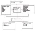
There is an almost unlimited manifold of mechanisms that lead to the failure of adhesive bonds (Scheme 1). Bond rupture can occur in adhesion or cohesion zones. Mechanical or chemical stress (or both) can cause bond failure. The last case seems to occur most often in a non-linear time dependency for the process of bond rupture.
Prediction of Bond Failure
Accelerated tests are used to predict the performance of adhesive bonds. During these tests, environmental conditions such as temperature, moisture, UV light or vibrations are enhanced in order to shorten the time frame for failure. For many of these tests, industrial standards are already in place, including tests for accelerated (forced) aging. The intrinsic problem with data collected under such conditions stems from the complexity of adhesive formulations. Adhesive systems have many degrees of freedom with respect to reaction pathways. The specific conditions under which the systems are aging will determine which kinetic pathways will take the lead. Consequently, the prognostic reliance of such tests depends on whether the same reaction mechanisms apply under forced conditions with respect to reality.
The lack of sufficient predictability of adhesive bonds is a source of great concern to many engineers. Unless the adhesive industry puts itself in a position to provide sound evidence and theoretical models pertaining to the life expectancy of adhesive bonds, engineers will continue to resort to alternative means, such as screws, rivets and bolts.
Influence of the Polymer Oxidation on Bond Stability
There can be many reasons for the mechanical breakdown of an adhesive bond; the long-term behavior of the polymers is perhaps the most difficult to predict. Oxidation processes leading to the cleavage of the polymer chains occur randomly and stealthily. They may not be detected for years, undergoing a rapid, autocatalytic acceleration once the reaction has reached a critical stage. Once the reduction of the molecular weight has reached a critical threshold, both adhesion and cohesion properties are critically affected, which, in turn, leads to a loss of required bond properties. Any method allowing meaningful prediction of the polymer aging in the solid state will therefore be most conducive to the evaluation of adhesive bonds.
Since most organic materials readily react with oxygen (even at ambient temperature), oxidative degradation is a severe problem in materials science. Monitoring what predicts the stability of polymeric materials against oxidation is, therefore, crucial. Commonly applied analytical methods such as measuring oxidation induction time (OIT) or oxidation onset temperature (OOT) using DSC or other conventional thermoanalytical methods are not suitable for long-term prediction of oxidative behavior because of the use of elevated temperatures during these experiments: the high temperatures may invoke reaction pathways that are different from those encountered under the conditions of use.
Determination of Oxidation Stability at Higher Temperatures
The oxidation of materials in the solid state generally starts on the surface, and the oxidation progress is mainly diffusion controlled. The general overview of commonly applied examination methods and the mechanism of oxidation is given by Feller,1 Zweifel,2 and Scheirs.3 Accelerated aging is normally initialized by extreme environmental conditions. During the induction period, stabilizers are consumed, while the organic matter remains stable, maintaining its original properties. At the end of the induction period, when the concentration of stabilizers reaches a sub-critical level, oxidative decay starts and the substance’s properties change. Frequently, oxidation reactions are self-accelerating (auto-oxidation) and the reaction progress may rapidly increase after the induction period.
The most common methods used to test the kinetics of thermo-oxidation of organic substances are thermal analysis methods like differential thermal analysis (DTA), DSC or TG. Substances are tested using isothermal or non-isothermal temperature profiles under an oxidative atmosphere, and the OIT or OOT are determined when the heat flow (DSC, DTA) becomes exothermal or the sample mass loss starts (TG). In some special applications, these procedures are standardized (such as for automotive oils, cable insulations or polyolefins).
OIT- and OOT-determination procedures are widely applied, especially for industrial and commercial applications. Their advantages include an easy sample preparation, short measurement periods and established methods of data evaluation. A significant disadvantage of these short-time experiments becomes apparent during the application of the high experimental temperatures, which are generally above 180°C. Such temperatures are used to ensure that the oxidation starts within two hours, and to provide a distinct signal that is larger than the baseline noise: the sensitivity of conventional thermal analysis instruments can be too low to record the beginning of the oxidation reaction at moderate temperature profiles. The evaluation of the bad correlation of OIT and OOT data with the observed long-term stabilities under normal environmental conditions is reported in references 4-6. Depending on the properties of the substance, one or several phase transitions can occur between the temperature ranges at which the oxidative characteristic has been measured, and those for which the oxidative properties has been predicted (lifetime determination). It seems obvious that degradation kinetics may change for different low- and high-temperature phases, and the extrapolation of high-temperature experimental results to ambient temperature can be of little value.
In this situation, the alternative methods, based on the experiments carried out at low temperatures, should be applied for the characterization of the long-term stability of organic substances.
Chemiluminescence
Luminescence is a term used for various phenomena, originating from electronically excited states. Luminescence is a “cold light,” not an incandescent light. The emission of photons results from the relaxation of excited electrons (triplet-state) into their ground state. This may be quite a quick process: the delay between excitation and light emission is at least 10-10 seconds. Chemiluminescence (CL) includes all luminescence phenomena resulting from chemical reactions.7 The fact that organic substances undergoing oxidation emit light was first recognized in the second half of the 19th century.8 In the past few years, chemiluminescence has gained wide acceptance as a sensitive method by which to study the oxidative degradation of organic solid substance.9-11
Principles of Chemiluminescence in Organics
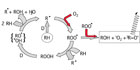
Light emission during the oxidative degradation process of organics is part of the reaction course. The first step is the formation of unstable alkyl radicals, which immediately scavenge the oxygen from the atmosphere to form peroxy radicals. These react further and transform into different species in an accelerating degradation cycle (auto-oxidation, see left part of Figure 1). This is normally attributed to a transition of excited triplet-carbonyl-functions (3R=O*) into their ground state. The spectral range of the light emitted varies according to the type of substances involved. In most cases, chemiluminescence is observed in the short wave region of the visible spectrum from 380 to 450 nm. However, there are well-known exceptions: the relaxation of 1O2 can be detected in the infrared region at ca. 1200 nm.
The energy required for this reaction (290-340 kJ mol-1) may be supplied by three different chemical mechanisms:
- The combination of two peroxy radicals with concomitant fragmentation in a Russel mechanism13 is strongly exothermal (460 kJ mol-1).14 The CL-emitter is an excited “triplet” carbonyl function (see right part of Figure 1).
- The direct homolysis of hydroperoxides followed by a cage reaction leads to an excited carbonyl-function and is combined with the evolution of 315 kJ mol-1.15
- The metathesis of alcoxy or peroxy radicals provides 374 kJ/mol and 323 kJ/mol, respectively.16 It has been shown that CL signal intensity reveals the existence of two kinetic stages during oxidative degradation of organic materials: the first one is correlated with the concentration of peroxide groups,17 while the second stage corresponds to the oxidation propagation by the hydrogen abstraction responsible for the carbonyl formation.18
Experimental Chemiluminescence Setup
The CL emission rate during oxidation of organic substances at ambient temperatures is too low to be detected. However, only moderate temperatures are required to provide detectable signals. The requirements for the oven used in this process are similar to those used in conventional thermoanalytical measurements such as DSC or TGA: exact control of the required temperature profile is a necessity, even in long-term experiments in a gas exchange facility. In addition, the sample compartment must be absolutely light-tight.
CL-emission detection may be achieved using a photomultiplier tube (PMT) with a photon counting mode or a slow-scan charged coupled device (CCD) camera. PMTs are highly sensitive devices that allow short gating times, but their dynamic ranges are low and their use must be carried out with caution in order to avoid the saturation of the photocathode. The advantages of solid-state detectors (CCDs) are their simplicity in use, their high dynamic range and the feature of imaging the sample to exhibit the inhomogeneous character of oxidation reactions. A third way of detecting CL emission is to use micro channel plates (MCP) or intensified CCDs. These sensors offer the best sensitivity in combination with the imaging facility, but are characterized by an exorbitant price, high operation complexity and a low dynamic range.
The instrumentations provided by AKTS-Chemiluminescence are fully automated and consist of thermoelectrically cooled PMT with a photon counting mode and an oven chamber in combination with an optical path including a shutter system (to protect the highly sensitive detection unit against extensive light during sample handling, as well as to provide background measurements). The single-cell instrumentation is designed especially for sensitive measurements at moderate temperature conditions (isothermal and non-isothermal mode), which allows experiments to be carried out under controlled relative humidity in temperatures up to 95°C. The multi-cell instrumentation enables the characterization/comparison of four independent samples at the same temperature profile without cross contamination.
Application of Chemiluminescence in the Investigation of Oxidation
In this study, we report on a new approach to kinetic analysis of the oxidation of organic solids at moderate temperatures using CL measurements carried out on newly developed instrumentation. The kinetic characteristics of the oxidation process calculated from the chemiluminescence signals are subsequently applied to the prediction of the reaction progress under different temperature profiles.
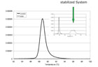
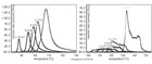
The presented results depict the comparison of the oxidation reactions of natural rubbers with and without stabilizer in an oxygen atmosphere. This system is representative of many hot-melt formulations, especially HMPSA. The results shown in Figure 2 illustrate the influence of the stabilizer (5% IrganoxTM 565) on the oxidation behavior of the rubber (cis-1,4-polyisoprene) during non-isothermal heating in the 30-120°C range with a rate of 0.0132 Kmin-1 in the oxygen atmosphere.
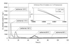
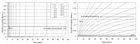
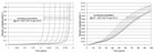
Having a set of experimental data under different isothermal conditions, an Arrhenius relationship can be evaluated (see Figure 3).
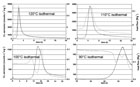
At higher temperatures (>100°C), the CL data corresponds well with the DSC data. When testing oxidative stabilities below 100°C, the limitations of conventional thermo-analytical methods such as DSC become obvious: useful evaluation of such data with regard to oxidation onset becomes tricky and is not reliable (see Figure 4).
Advantages of Chemiluminescence in Monitoring Oxidation of Organics
Compared to DSC and other conventional thermo-analytical methods, CL offers many advantages. Due to its much higher sensitivity, experiments can be performed at much lower temperatures (i.e., closer to application-related conditions). This fact is essential to the characterization of substances with low-temperature melting points, glass transitions, etc. The outstanding baseline stability of CL is of great benefit when performing long-term experiments 19; moreover, the CL-signal is exclusively related to the oxidation processes and is therefore not superposed by signals resulting from other reactions, including phase transitions. The instrumentation setup may be designed individually for special fields of application and goals of research. The experiments can be performed with sample masses as low as approx. 0.1 mg. A basic instrumentation would not be any more expensive than a commercial DSC apparatus.
Application of an Advanced Kinetic Analysis of CL Signals for Lifetime Prediction
Determination of Kinetic Parameters – Isoconversional Analysis
The noticeable weakness of the ‘single curve’ methods (determination of kinetic parameters from single runs recorded with one heating rate or isothermal condition only) has led to the introduction of ‘multi curve’ methods over the past few years, as discussed in the International ICTAC kinetics project.21- 24 Degradation reactions are often too complex to be described in terms of a single pair of Arrhenius parameters and the commonly applied set of reaction models. As a general rule, these reactions demonstrate multi-step characteristics. They can involve several processes with different activation energies and mechanisms. In such situations, the reaction rate can be explained only by complex equations where the activation energy term is no longer constant but is dependent on the reaction progress (E ≠ const but E = E(α)).
Isoconversional methods were introduced by Friedman25 and Ozawa-Flynn-Wall.26, 27 A detailed analysis of various isoconversional methods (i.e., the isoconversional differential and integral methods) for the determination of activation energy has been presented by Budrugeac.28 The convergence of the activation energy values obtained by means of a differential method (Friedman) with those resulting from the use of integral methods (Ozawa-Flynn-Wall) comes from the fundamentals of the differential and integral calculus.
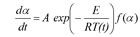
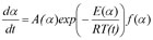
The differential isoconversional method of Friedman is based on the Arrhenius equation
with
f(α): the model function
A: the preexponential factor
E: the activation energy
T: the temperature
t: the time
Friedman has applied the logarithm of the conversion rate da/dt as a function of the reciprocal temperature at any conversion a:
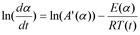
As f(α) is a constant in the last term at any fixed a, the logarithm of the conversion rate da/dt over 1/T shows a straight-line dependence with the slope of m = -E/R.
By the extension of the expression

With
A'(α) = A(α) f(α)
one can predict the reaction rate or reaction progress having determined A'(α) and E(α) using the following expression:
at any temperature profile such as isothermal, non-isothermal, stepwise, modulated temperature or periodic temperature variations, etc.
Kinetic Description of the Oxidation of Natural Rubber
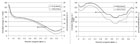
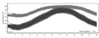
The CL signals collected during the oxidation of unstabilized and stabilized natural rubber under non-isothermal conditions at different heating rates were used for the determination of kinetic parameters later used for the prediction of the reaction progress. The normalized reaction rates determined by AKTS-Thermokinetics software are depicted in Figure 6.
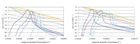
Once the kinetic parameters are determined, they can be applied to predict the course of oxidation under different temperature profiles. The presented results clearly indicate the oxidative induction period after which the rate of oxidation accelerates rapidly. The prediction of the oxidation of the natural rubber under isothermal conditions at low temperatures (4-40°C) is shown in Figure 7.
The most important goal in the investigation of the kinetics of thermal decomposition is the determination of the thermal stability of substances (i.e., the temperature range over which a substance does not decompose at an appreciable rate). The correct prediction of the reaction progress of materials that are unstable under ambient conditions requires accurate calculation of both kinetic parameters and the exact experimental temperature profile.
The example showing the prediction of the properties of rubber under a more complicated temperature profile is illustrated in Figure 8, which presents the oxidation progress of natural rubber at 20°C when the temperature changes with the modulations of 0, 5, 10 and 20 K each 24 h. The dependences shown in Fig. 8 indicate that even small temperature fluctuations can significantly change the stability of the substance (e.g., the amplitude of 10K at 20°C lowers the oxidation stability of natural rubber by half of lifetime).
In general, calculations can be achieved for any fluctuation of temperature that makes the prediction of thermal stability properties for varying climates possible.
Exact consideration of the calculations of daily minimal and maximum temperature variations of worldwide climates therefore provides very valuable insight when interpreting and quantifying the reaction progress of materials subjected to atmospheric conditions.
Conclusion
Oxidative degradation of polymers can be monitored by the chemiluminescence method. This method is an order of magnitude more sensitive than conventional methods of thermal analysis such as Differential Scanning Calorimetry, Differential Thermal Analysis or Thermogravimetry. The data acquired during the chemiluminescence experiments carried out iso- or nonisothermally can be evaluated by differential isoconversional kinetic analysis to obtain meaningful and accurate predictions of the lifetime of organic materials in temperature domains that are representative of the life-cycle of the planned products. Within the same context, the efficiency of stabilizers or influence of environmental factors such as relative humidity, UV-radiation and pollutants can be forecast.

The equipment used for the data collection was developed by AKTS-Chemiluminescence. This is a powerful tool, fully automated and supported by user-friendly yet powerful software. It enables formulators of adhesives and coatings to evaluate their products with respect to oxidative aging in order to make meaningful predictions of the aging behavior.
For more information on age simulation, visit www.collano.com or www.akts.com.
Links
Looking for a reprint of this article?
From high-res PDFs to custom plaques, order your copy today!


