A Sticky Optimization
Technical professionals in the pressure-sensitive adhesives area are highly skilled and educated in tape-making processes. They have often taken course-work in the areas of PSA tape properties, characteristics of tape-making, web-handling, coating and converting processes. Subject-matter knowledge is generally abundant. This article demonstrates a statistical methodology that builds on subject-matter knowledge to objectively fine-tune both processes and product formulations. The method will be illustrated with a case study where the experimenter was trying to optimize an adhesive to achieve specific test properties.
What methods are currently used for process optimization? How does one find the ideal settings when there are competing criteria? Design of experiments (DOE) is a formalized method of data collection and analysis. Computer technology has turned what used to be a series of tedious mathematical calculations into fairly quick, yet sophisticated, analyses. From these analyses, a subject-matter expert can optimize process settings by making knowledgeable tradeoffs in the response criteria. DOE can be used both in laboratory research and on the manufacturing plant floor.
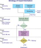
Researchers and engineers who are unfamiliar with DOE can be overwhelmed by the number of design options. Designed experiments can be run to accomplish many goals. The right design must be chosen to meet the objective of the problem. Figure 1 illustrates how the objective of the design determines the type of design chosen. The discovery phase uses screening designs to identify the primary factors that control the system. These designs are especially helpful to quickly sift through a large number of possible factors whose true contributions to the system are not understood. Typically, two-level fractional-factorial designs are used in this phase, preferably something called a Resolution IV design.1 The breakthrough phase uses either full factorial or slightly fractional factorial designs (Resolution V or higher) to positively identify both main effects and interaction effects. At this point, center points may also be added to the design in order to determine if any quadratic effects might be present. The optimization phase is required when at least some of the factors have a curvilinear relationship with some of the responses. It uses response surface designs, such as central composite (CCD) and Box-Behnken (BB) designs.2 Lastly, validation runs finalize the DOE process by confirming the results in a longer-term setting.
Case Study
A client manufacturing an adhesive wanted to ensure that the final adhesion properties could be consistently achieved. This entailed identifying optimal processing conditions. Preliminary work determined that there were three key factors that were critical to the manufacturing process. The names of these factors have been removed to protect proprietary information. The engineer responsible for the process decided that he needed to run a designed experiment with the goal of process optimization. This goal meant that a response surface design was in order.Two standard response surface designs3 are central composite designs and Box-Behnken designs. This client chose the Box-Behnken design because each of his three factors could be easily set to the three levels required by the design. The total number of runs is 17, which was deemed reasonable by the manufacturing personnel. The design is shown in Table 1. The runs are physically completed in the random run order. Notice that the design includes five center points that are randomly scattered throughout the other runs.
Product samples were made at each of the 17 sets of conditions. The laboratory then measured seven key quality characteristics, including some viscosities, tensiles, and subtak and subadhesion properties. This data was entered into a statistical software package4 that can perform an analysis of variance in order to establish a polynomial prediction equation for each response.

Sample Data Analysis
The analysis of data from a designed experiment is done using a statistical tool called analysis of variance. Table 2 illustrates an example of the analysis of one of the responses in this design - Tensile at 0 day. Without going into all the details of how this analysis is created, it is more important for an experimenter to understand how to interpret the information presented.The p-value is the primary column of interest. It quantifies how significant each term is in the polynomial model. A smaller number is better, and as a general rule of thumb, terms are considered statistically significant when their p-value is 0.05 or lower. In this case all but one of these terms is substantially lower than 0.05. You might notice that the AC term is missing. This term had a p-value significantly higher than 0.05, so it was removed from the model.
In addition to the p-values, the R-squared values given in the lower part of the table are also of interest when a response surface design is run. The R-squared represents the amount of variation in the data that is explained by the model. The predicted R-squared represents the amount of variation in predictions that is explained by the model. When the objective of the experiment is to optimize, higher R-squared values are important, implying that the polynomial model is a very good predictor of the response. The higher the R-squared values are, the better the polynomial is at either describing the system or making predictions about the system. For this response, the R-squared values of approximately 98-99% indicate that this polynomial is a very good description of the relationship between these three factors and the Tensile at 0 day response.
Sample Graphical Analysis
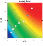
The statistical analysis should be validated by an examination of residual diagnostics plots. This step is not illustrated here, but should not be overlooked. Typically, the experimenter would confirm that the studentized residuals follow a normal distribution, and that they have a constant variance. Also, the data should be checked to make sure it contains no discrepant values. After the diagnostic validation step is complete, graphical illustrations of the model can be produced, as shown by the contour plots in Figure 2.These contour plots have X1 on the horizontal axis and X2 on the vertical axis, with X3 fixed at a specific level (in this case, the low and high levels of 5 and 20). Tensile at 0 day predicted contours fill the graphical area. According to the experimenter's subject matter knowledge, the optimal response value is 65. Notice that on the left-hand graph, there is a contour line labeled "65" that cuts through the middle of the graph area. When X3 is set at its low value of 5, any of the combinations of X1 and X2 settings that fall on that 65 line would be feasible. Now the X3 factor is moved to its high setting of 20 and the right-hand graph shows the line for "65" falling closer to the lower-left corner.

Multiple Response Optimization
Typically, the quality of a product is measured by many different quality characteristics. This case study has seven different responses, each of which is modeled with a different polynomial equation. Some models will be linear (containing only terms such as A and B), while others are quadratic (containing squared terms to model non-linearity). Accordingly, each will have different contour plots with differing "optimal" factor settings. Working through these graphs by hand for seven different responses can be a very time-consuming and inefficient process; it is also prone to mistakes. Statistical software packages typically have a mathematical multiple response optimization routine. This is a method of pulling together all the polynomial models and determining a set of conditions that is a compromise to all the stated goals.Table 3 shows a summary of all seven responses, the terms that were significant in their models and summary statistics for each model. Typically, some of the responses will fit to polynomials better than others. In this case, Tensile at 0 day fits almost perfectly, while Subadhesion does not fit as well, but is still adequate.
After the analysis of each response is complete, these models are used in the numerical optimization routine. This case study uses the optimization criteria in Table 4. The goal is the targeted value, but it is surrounded by an acceptable range that is defined by the low and high values.
The "sweet spot" in processing conditions that achieves all the goals for this adhesive is shown in Figure 3, which displays factors X1 and X2, with X3 set at its low level of 5.
The client may have stumbled upon this set of operating conditions by chance, but it is unlikely that they would have had a clear picture of which responses define this region. It turns out that the left side of the operating window is defined by the initial viscosity limit of 55,000. The bottom is defined by the viscosity at 50%, and the right side is defined by both the subtak at 0 day and the tensile at 3 day. If the limits of any of these can be expanded, then the operating region will open up. This is a critical gain in process understanding, because it also indicates that the other responses do not control the operating conditions.
Summary
Design of experiments (DOE) can be a challenge to implement because it differs from traditional one-factor-at-a-time experimentation. Old habits don't necessarily fit into the "DOE way" of doing things. DOE adds tremendous efficiency to understanding how processes work. It allows complex processes to be broken down so that they can be understood as a group of interacting factors.This was simply one illustration of the use of design of experiments. Two-level factorial DOE can be used to identify which variables in a process are critical to control. Mixture designs are used to optimize a chemical formulation to meet specific criteria. Robust design helps find factor settings that make a product or process robust to variations in uncontrollable variables.
Technical professionals will find many ways to apply design of experiments. It just takes a little education and a bit of practice to discover that experimentation can be done on a whole new level.
This article is based on a paper presented at the Pressure Sensitive Tape Council's Tech XXVII Technical Seminar May 4-6, 2005.
For more information on design of experiments, contact Shari L. Kraber, MS Applied Stats, PE, CQE, Statistical Consultant, Stat-Ease Inc., 2021 E Hennepin Ave, Suite 480, Minneapolis, MN 55413; e-mail shari@statease.com; or visit www.statease.com.
Looking for a reprint of this article?
From high-res PDFs to custom plaques, order your copy today!


