Digitalization and Predictive Modeling of Polyurethane Data

Data is being collected at an unprecedented rate, and this trend will only increase into the future. This data-centric paradigm shift is happening in all areas of society, and the chemical sector is no exception. Chemical data from a variety of sources is being collected from many areas of the sector, including research and development, business, scale-up, and production. Digitalizing this data (i.e., moving from pencil and paper lab notebooks to electronic lab notebooks, databases, and so on) offers many advantages, including providing a sustainable medium through which to store and reference information, preventing double-work, and offering the opportunity for data science.

This latter approach utilizes statistics to learn from the data and make predictions. Machine learning (ML) and artificial intelligence (AI) are powerful, emerging technologies that can take data and determine complex relationships between inputs and outputs, thereby offering a route to improve and optimize materials and chemicals.

The ability to properly learn from data and employ ML and AI is not trivial. The task often encounters many challenges, including large volumes of data, data uncertainty, and the complex nature of data. However, the development of predictive and flexible algorithms, coupled with computational power, has provided an opportunity to tackle these challenges.

One particular chemistry in which ML can be advantageous is polyurethane (PU) slabstock foam applications. These are flexible polyurethane foams that are used in products ranging from furniture to mattresses. Polyurethane chemistry is complex, with many formulation components dictating the ultimate foam properties. These components include polyols, isocyanates, surfactants, and catalysts, just to name a few.

Furthermore, consumers require tight specifications on the resulting slabstock foam properties (density, hardness, etc.). It often takes many years to develop the expertise to understand this complex relationship. However, customers are demanding more innovative products, faster development, and quicker technical service. It is often challenging to meet these expedited timeframes with the “old-fashioned” way of performing experiments. Because of this, machine learning is a way to meet these challenges, even with complex chemistry.

Herein, we will show how ML was applied to slabstock foam data in order to accelerate development and guide decision making. Flexible polyurethane foam data was collected from years of previous formulation work. ML algorithms were applied to this data to generate predictive models, and with these models both predictions of the foam properties (forward models), as well as predictions of formulations leading to targeted properties (reverse models) can be done.

Experimental

Data was collected from pilot-scale flexible foam operations at BASF’s Wyandotte facility. Two main clusters of data included the foam recipe data and the foam performance property data. The former, stored as csv files, was collected directly from the Cannon Viking CarDio Pilot Slabstock machine. This data set included five years’ worth of formulation data, listing the type and amount of each component used to make individual foams. Coupled to this were the physical testing data for each foam.

The goal of this work is to map the foam formulation components to the physical properties of the foam. In terms of nomenclature throughout this article, factors and x-variables are used interchangeably (these are the independent variables); responses and y-variables are also used interchangeably (these are the dependent variables). Together, there were 1,778 records (foams), 96 factors (formulation components), and four responses (foam properties).

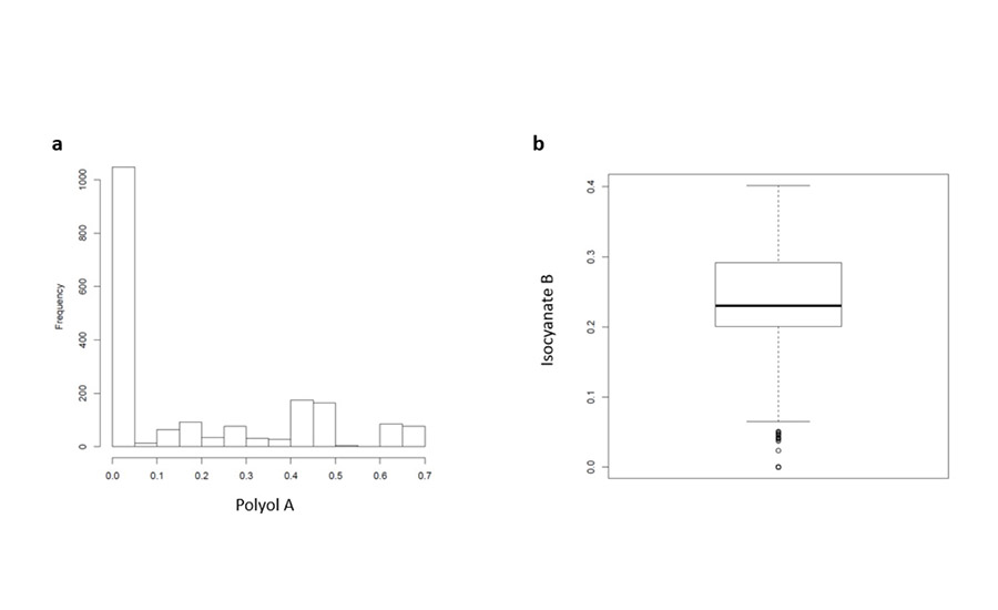
Prior to modeling, exploratory data analysis (EDA) was performed. In this step, various statistical and graphical approaches are applied to the data in order to get a better sense of its makeup. While there are many approaches to EDA, an example of visualizing the data spread through two means is shown in Figure 1.

*Click the image for greater detail

Figure 1. Example of exploratory data analysis performed on slabstock foam data: histogram (a) and boxplot (b), showing the spread of a given polyol and isocyanate, respectively.

After exploratory analysis, modeling work commenced. First, the data were split into a training and test data set. 75% of the data set was randomly chosen to be used to train the models; the remaining 25% was used to test the accuracy of the final models. This hold-out test set is needed in order to obtain an unbiased measurement of model performance.

The factors were standardized by centering and scaling: the values of each column were subtracted by the column mean; the difference was divided by the column standard deviation. This standardization helps to make all of the factors on the same “scale,” so that the magnitudes of the factors don’t dictate their significance. This is especially important when performing statistical tests on factor effects in linear models.

In addition, the responses were logarithmically transformed. While this was not initially done, the necessity of this step was determined through residual analysis of the ordinary least squares (OLS) models and outliers. In OLS, the residuals of the model (difference between the model and experimental data) should show homoscedasticity (i.e., the variance of the error term is the same for all observations). If this is not the case, several methods can be employed to deal with heteroscedasticity, including transformation to achieve constant variance. Furthermore, logarithmically transforming the response variables can help reduce the effect of leverage points, which can skew the model, particularly if the leverage point is an outlier.

From here, various empirical (data driven) models were trained. Except in special circumstances, it is difficult to judge which statistical or machine learning model will be the best when modeling a given data set. Therefore, 10 machine learning models were trained on the training set for each of the responses of interest.

In all modeling approaches, hyperparameters were first tuned. Hyperparameters are adjustable parameters in a model algorithm that guide the variance/bias tradeoff. For example, the elastic net has λ1 and λ2 as hyperparameters, while the cubist has the number of committees and nearest neighbors as hyperparameters (elastic net and cubist will be discussed more in depth later).

Overly complex models have high variance and low bias; the opposite is true for overly simple models. One would like the best of both worlds, which is often found when prediction error in a hold-out data set is minimized. In practice, this is done through cross-validation. For each response, fives repeats of a five-fold cross-validation were performed to determine the optimal hyperparameter values for each model. The algorithm for cross-validation is:

For i = 1: number of hyperparameter combinations

Set hyperparameters to combination i
For j = 1:5
Set random seed
Split training setup into five equal parts
For k = 1:5
- Remove kth part of the training set
- Train the model on the remaining four parts
- Predict data in the kth part, and record root mean squared error (RMSE)

Choose hyperparameter combination that minimizes RMSE

After the hyperparameters were determined for each model, the models themselves were compared via their cross-validation error. The algorithm that led to the lowest cross-validation RMSE was then chosen as the final model. Interpretation can be challenging for highly non-linear and non-parametric models, lending to the name of “blackbox” models.

While the mapping between inputs and outputs can generate accurate predictions, understanding how the inputs affect the outputs can often not be obtained easily with these models. As a result, several methods were employed to aid in interpretability. Partial dependence plots (PDP) show how a given output variable changes when varying a given input variable, calculated from the model at an average value of all other input variables. Individual conditional expectation (ICE) plots display this same trend of x vs. y. However, instead of averaging the rest of the input value prior to calculation, multiple curves are displayed, representing each data point in the data set.

In addition to overall trends, one may want to determine which factors are the most influential input variables guiding a model prediction. For instance, if the model predicts that, for a given formulation, the density will be 1.9 pcf, a pertinent question would be why 1.9 was obtained and to which formulation components the density was most sensitive. To this end, LIME (local interpretable model-agnostic explanations) was implemented. The LIME algorithm creates a simple-to-interpret linear model around the prediction of interest, no matter how complex the underlying model is. From this linear model, simple coefficients plots are outputted, from which variable sensitivities can be easily extracted.

Once the models were generated for each response, an optimization algorithm was utilized in order to solve the “reverse” problem. The previously discussed models predict foam physical properties based on a given formulation composition. It is often desired to reach a target property, with the question being how to get there. This was done through mathematical optimization. Numerous optimization algorithms are available, each with pros and cons.

Differential evolution (DE) was employed for the current models. DE is an approach to (and associated algorithm for) optimization, falling into the class of evolutionary algorithms. These algorithms do not rely on gradient information but instead improve the objective function in a series of iterations in which the decision variables “evolve” through various rules and heuristics.

This approach was used to optimize slabstock foams. One can specify which foam properties are of interest, as well as their desired values (e.g., target, minimize, maximize). In addition, one sets the decision variables (i.e., which formulation components one wants to vary in order to obtain the desired properties) and their ranges.

Exploratory data analysis, model training, model interpretation, and optimization were done in R1, version 3.5.2. R is a programming language that specializes in statistical analysis and computing. Many R packages are available to perform a wide range of tasks, from visualization to machine learning. The main packages used for the present work include: ggplot2 (visualization); caret, cubist, and elastic net (model training); PDP, LIME, and tSNE (model and data interpretation); and DEoptim and desirability (optimization).

Results and Discussion

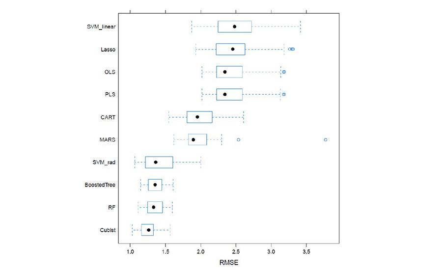
After data cleaning and preprocessing, numerous models were trained and compared as previously described. Figure 2 shows the comparison of these models by their cross-validation error. The cross-validated (fives times a five-fold CV) RMSE for each model is represented as a box plot. The most predictive model is expected to be the one with the box plot farthest to the left (i.e., with the lowest RMSE). Furthermore, a small boxplot represents a low spread of the errors (which is favorable).

*Click the image for greater detail

Figure 2. Comparison of cross-validated RMSE across numerous machine learning models for the response of density.

Figure 2 shows the cubist model having both the lowest CV RMSE, as well as small RMSE spread. This conclusion was consistent throughout all responses of interest (i.e., the cubist model was the most appropriate for all responses).

Cubist^2,3,4 is based on classification and regression trees (CART), a powerful machine learning method that generates decisions based on binary splits in the x-variable space. Cubist offers improvements over the standard CART algorithm. First, along with other methods (e.g., random forest), it creates ensembles of trees, called committees. Second, it employees nearest neighbor corrections. Finally, it utilizes regression at the leaves. In typical tree-based models, the leaf (prediction) of the model is a single value. With cubist, it is not a single value; the prediction is made through a simple linear regression model.

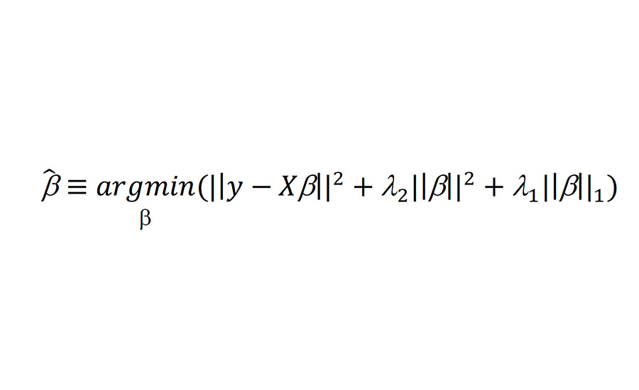
Because of the complex nature of the cubist model, it was also prudent to implement a second model that is more interpretable. The selected model for this purpose was the elastic net, a regularized linear model approach combining the benefits of two regularized approaches: ridge regression⁵ and LASSO⁶. The former regularizes based on the L2 norm, and the latter based on the L1 norm. Combining these leads to the following formulism:

*Click the image for greater detail

Elastic net offers several advantages, the most powerful of which is automatic feature selection. With regularization, the approach shrinks the coefficients in order to minimize cross-validation error. When the model coefficients approach 0, the term is removed from the model. Furthermore, because the final model is a linear one, elastic net models are quite interpretable.

These two algorithms were used to train the data sets to obtain the final models for each of the foam properties of interest. Once the final models (and associated hyperparameters) were developed on the training data set, they were applied to the test data set, which was not used to train the models. This is an important check for predictivity; the model should be able to accurately predict data points that were not present during model training.

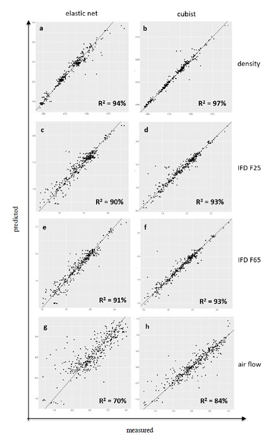
Figure 3 shows the predictions of these models on the test set. Each predicted property has two sets of predictions: one using the cubist model, and one using the elastic net. The parity plot for each combination is shown, displaying the measured values (x-axis) vs. the predicted values (y-axis) of the test set data. A perfect fit would fall directly on the x=y line. R2 are also shown for each set of predictions.

*Click the image for greater detail

Figure 3. Test set parity plots for the four responses (density: a, b; IFD F25: c, d; IFD F65: e, f; air flow: g, h), modeled with either elastic net (a, c, e, g) or cubist (b, d, f, h).

As shown, the models do an excellent job of predicting the hold-out test set. The most accurate of these predicts the density with an R2 of 97%, meaning that 97% of the variation is explained by the model. Air flow was more difficult to predict, but even this had an R2 of 84%. It is interesting to note that, with the exception of air flow, the linear model (elastic net) is only slightly worse than the non-linear model (cubist). This suggests that linear terms are most influential for density and hardness.

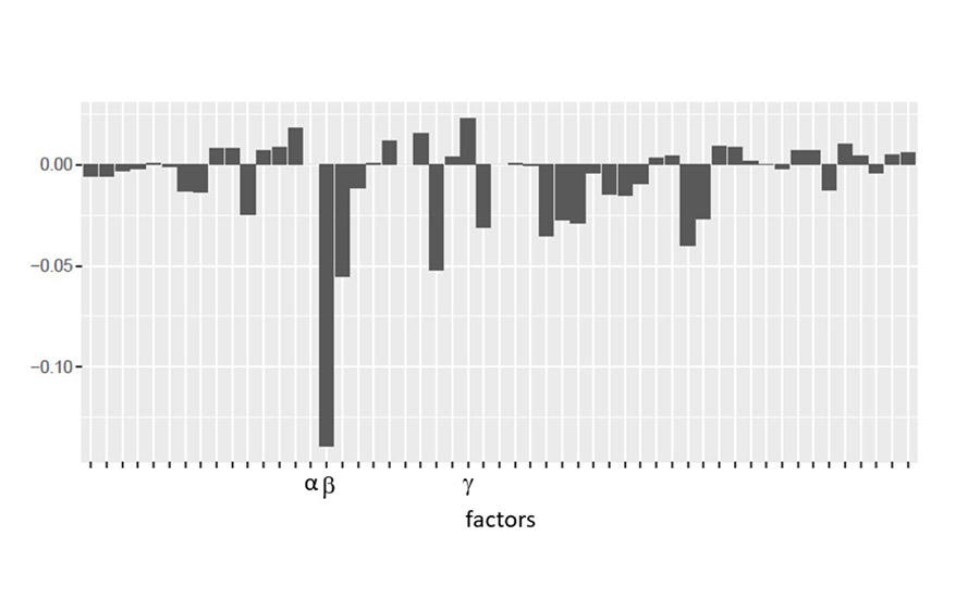
As a regularized linear model, the elastic net has the advantage of highly interpretable terms. By analysis of the term coefficients, one can obtain a measure of the variable’s sensitivity (coefficient magnitude) and directionality (whether the coefficient is positive or negative).

Figure 4 shows the coefficient plot for the response of density. This shows that variables such as α have a negligible effect on density, while factor ß is highly negatively correlated with density and factor γ is positively correlated with density. It should be noted that these conclusions are based on a linear model and as such might not be completely accurate, given that the process could show at least some non-linear trends.

*Click the image for greater detail

Figure 4. Coefficient plot for the density elastic net model.

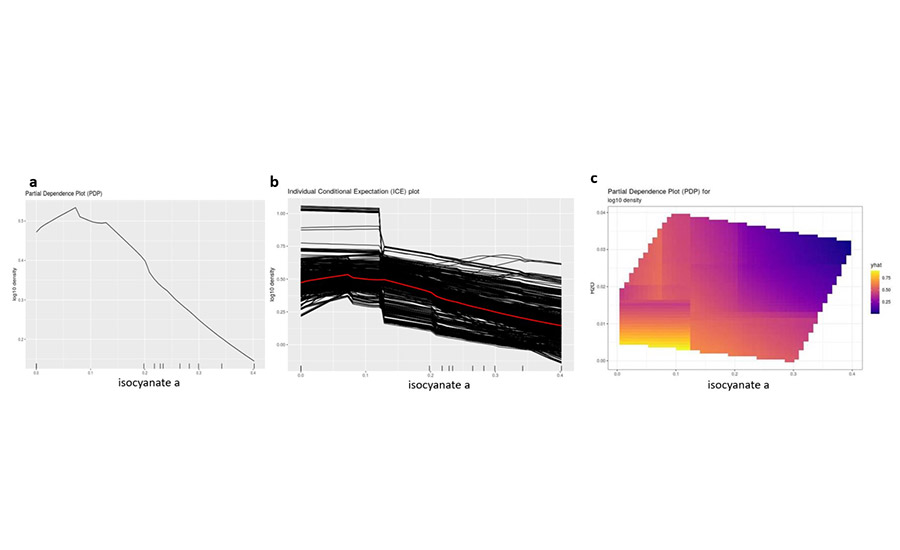
To circumvent this limitation of the coefficient plot being applicable to only linear models, the PDP and ICE approaches were applied to the highly non-linear cubist model. These provide a visualization of how input variables affect an output variable across the input variable’s range.

An example of this visualization when applied to an isocyanate’s effect on density is shown in Figure 5. These representations show that as the isocyanate increases, density decreases. However, non-linearities can be observed; for instance, for up to 5 wt% of the isocyanate, there is actually a slight increase in density with increasing isocyanate (average effect over all other variable values).

*Click the image for greater detail

Figure 5. Partial dependence plot (a) and individual conditional expectation plot (b) of an isocyanate on density; partial dependence plot (c) of an isocyanate and water on density.

For the PDP approach, one can extend this analysis to examine two variables at a time, which helps in understanding synergistic and antagonistic effects of the variables on the response. This behavior is shown in Figure 5c, displaying both the isocyanate’s and water’s effect on density. In addition to assisting in understanding the trends in the model, this can help in gaining a more holistic view of how the formulation components contribute to foam properties.

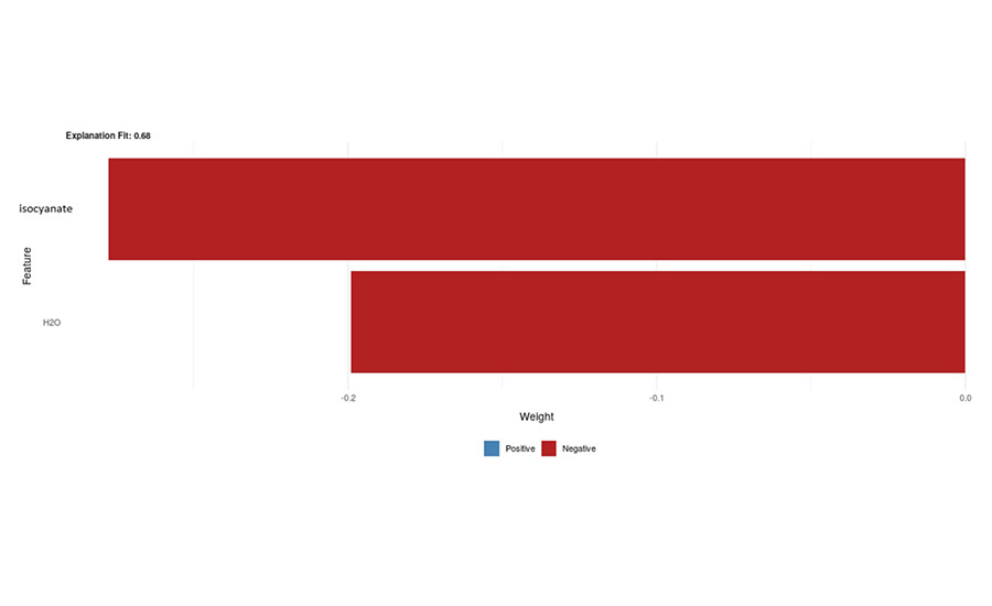
To further understand how the model predictions are generated, LIME was integrated into the workflow and can be applied to any prediction made by the model. As described previously, this approach fits a linear surrogate model to a given prediction, thereby providing a simple-to-understand representation of the main factors guiding a foam property. Figure 6 is an example of this LIME representation for a density prediction of 2.1 pcf resulting from a mixture of a polyol, several amine and tin catalysts, a surfactant, an isocyanate, and water.

*Click the image for greater detail

Figure 6. Example of a LIME representation of a density model prediction.

The LIME plot shows the biggest drivers are the latter two components and that they have a negative correlation with the response. This agrees with the PDP plots (Figure 5). Also, as shown, this representation accounts for approximately 70% of the model fit.

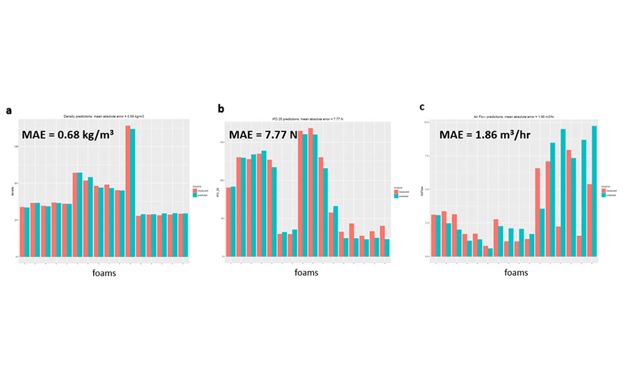
As a final test of the model accuracy, the models were applied to a “future” data set, completely outside of the timeframe of the training data. The models were trained on foam data coming from 2012-2017. While the test set was held out during training and therefore was not seen by the algorithms, it still came from the same time range. As a further check, new data was used, coming from foams synthesized in 2018. The models were applied to this “newer” data set: the formulation data from the 2018 foams were the model inputs, with the outputs being the foam properties. The results for the prediction of density, IFD F25, and airflow are shown in Figure 7.

*Click the image for greater detail

Figure 7. Comparison of the measured (red) and predicted (teal) foam properties (a: density; b: IFD F25; c: air flow) for various foams synthesized in 2018. The mean absolute error (MAE) is shown for each set of predictions.

As one can see, the predictions are quite accurate, with little deviation between the measured and predicted properties. There are a few exceptions, notably the air flow properties of several foams (the relative difficulty in modeling air flow is also seen in Figure 3). However, these deviations are more the exception than the rule; the majority of foams show excellent agreement between measured and simulated values. This further shows the effectiveness of the models to predict foam properties, even with “future” formulations not directly made during the model training.

These predictive models were used in the next step of the digitalization process: the reverse engineering of flexible foams. This is often the ultimate goal of most machine learning approaches: determining which input variables can achieve a target property (or properties) of interest. Though it is an inherently more challenging problem and requires both “forward models” (like machine learning models), as well as the appropriate optimization algorithm, it has the opportunity to provide great returns.

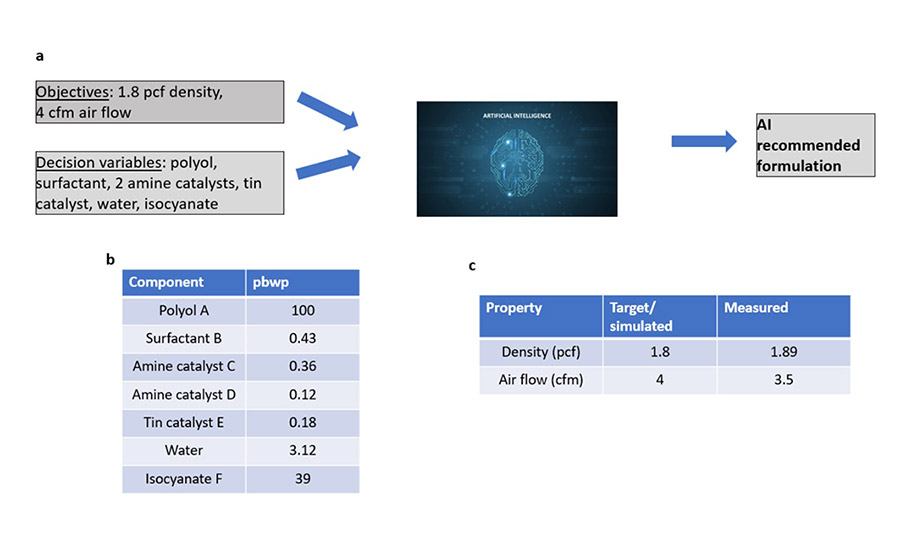
As described previously, the differential evolution algorithm was used to mathematically optimize the foam property machine learning models, incorporating decision variables (i.e., which formulation components to tune), constraints, and foam property targets. Figure 8 illustrates an example of the optimization framework, along with the resulting optimized foam and suggested formulation. In this example, the objective was to obtain a foam with 1.8 pcf density and 4 cfm air flow. Furthermore, we would like to achieve this by adjusting polyol A, surfactant B, amine catalysts C and D, tin catalyst E, water, and isocyanate F (as shown in Figure 8a).

*Click the image for greater detail

Figure 8. Approach to leverage computer-aided formulation suggestions (a); suggested formulation based on the targets of interest (b); comparison of measured and target foam properties (c).

The differential evolution algorithm was run using these objectives and decision variables. It should be noted that trying to optimize more than one response is not a trivial task. Often, one has competing targets and cannot hit the targets of more than one property simultaneously.

There are numerous ways to tackle multi-objective optimization. In this implementation, desirability functions were utilized. This approach allows for the combination of multiple targets into one objective function and enables one to set weights to different responses. When applying this methodology, the optimization algorithm provided suggested formulations to achieve these targets (one of these suggested formulations is shown in Figure 8b) and the predicted properties (see Figure 8c). This recommended formulation was run in the lab, and analytical measurements were done on the resulting foam (also shown in Figure 8c).

The results are encouraging. The measured density and airflow are close to the target, with deviations ranging from approximately 5% (density) to about 14% (for air flow). This demonstrates the usefulness of the “inverse model” in guiding experiments and providing suggested foam formulations to reach desired properties.

When performing optimization, one must pay special attention not to extrapolate. Without care, the optimal solution may reside in an area of the “data cloud” that is sparsely populated (i.e., where there is not much training data). While empirical approaches are good at interpolating, extrapolating can lead to inaccurate results.

To mitigate extrapolation, constraints have been included into the optimization framework. These include box constraints (minimum and maximum values for each decision variable), as well as linear constraints (ranges of combinations of variables). Constraints can be subsequently added as needed.

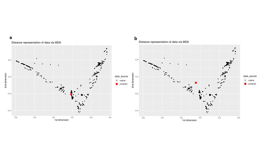
Extrapolation can also be mitigated by visualizing where a given prediction resides with respect to the data in the training data set. This is challenging, though, given the high dimensionality of the data. Because of this, two methods to easily visualize the data cloud and any incoming predictions were employed: multidimensional scaling (MDS) and t-distributed stochastic neighbor embedding (tSNE). Both methods visualize high dimensional data in a 2- (or 3-) dimensional way, such that points close to each other are close in the higher dimensional space. MDS is a linear method, while tSNE is a non-linear method.

Figure 9 shows a set of MDS visualizations, with the black dots representing the training data in a 2-dimensional plot. In Figure 9a, the red dot denotes a new formulation that is similar to the training data. In this case, the user can be more confident that the model will not be subject to extrapolation. Conversely, Figure 9b shows a new formulation that seems to be quite dissimilar to the training data. In this latter case, the user should be mindful of possible extrapolation and not rely too heavily on that particular model prediction.

*Click the image for greater detail

Figure 9. MDS representation of the training data, with a new prediction lying close (a) and far (b) from the original dataset.

Conclusion

A digitalization framework was applied to polyurethane slabstock foams. Machine learning models were trained on structured foam data consisting of formulation information and foam properties. These machine learning models are able to accurately predict foam properties of density, airflow, and hardness from the formulation.

Various methods were employed to gain insight into these models and to gain a better understanding of flexible foam chemistry. Beyond foam prediction, machine learning and optimization were applied to reverse engineer foams. These tools allow non-data scientists to utilize advanced machine learning to accelerate development of slabstock foams and drive innovation. This modeling methodology has been proven to be successful with flexible foams, which is the hardest application; therefore, we are confident it can be applied in other PU technologies.

For more information, visit www.basf.com.

“Digitalization and Predictive Modeling of Polyurethane Data,” 2021 Polyurethanes Technical Conference 05-07 October 2021, Denver, Colo., USA, Published with permission of CPI, Center for the Polyurethanes Industry, Washington, DC

References

R Core Team, “R: A language and environment for statistical computing,” R Foundation for Statistical Computing, Vienna, Austria, 2019, https://www.r-project.org/.
R. Quinlan, “Simplifying Decision Trees,” International Journal of Man-Machine Studies, 1987, 27(3), 221-234.
R. Quinlan, “Learning with Continuous Classes,” Proceedings of the 5th Australian Joint Conference on Artificial Intelligence, 1992, 343-348.
R. Quinlan, “Combining Instance-Based and Model-Based Learning,” Proceedings of the Tenth International Conference on Machine Learning, 1993, 236-243.
5.A. Hoerl, “Ridge Regression: Biased Estimation for Nonorthogonal Problems,” Technometrics, 1970, 12(1), 55-67.
R. Tibshirani, “Regression Shrinkage and Selection via the lasso,” Journal of the Royal Statistical Society Series B (Methodological), 1996, 58(1), 267-288.